NOVA: Fundamental Limits of Knowledge Discovery Through AI

Chapter One

The Central Question

Corresponds to Section 1 of the paper

Can AI systems discover genuinely new knowledge through iterative self-improvement, and if so, at what cost? Recent systems have begun to answer this empirically: AlphaProof achieved silver-medal performance at the International Mathematical Olympiad, DeepSeek-Prover-V2 advanced formal mathematical reasoning, and STaR demonstrated that models can bootstrap their own reasoning capabilities.

These successes share a common architecture: a model generates candidate artifacts, a verifier filters for correctness, and the verified outputs are fed back to improve the model. This "generate, verify, accumulate, retrain" loop is emerging as the dominant paradigm for AI-driven knowledge discovery.

Yet despite these empirical advances, we lack a theoretical understanding of the fundamental limits of this process. The NOVA framework addresses six foundational questions:

Core Questions

(1) How fast can an AI system discover new knowledge, and at what cost? (2) Does the rate of discovery inevitably slow down, and if so, how severely? (3) Under what conditions does the process converge to the target knowledge domain? (4) When does it collapse? (5) What role does verification quality play? (6) Can AI bootstrap itself to discover all knowledge autonomously, or is human guidance fundamentally necessary?

The paper introduces NOVA (Navigating the Origins and Verification of AI Knowledge) to provide the first rigorous theoretical foundation for these questions, connecting the problem to species estimation, occupancy laws, and support-limited sampling.

Chapter Two

Problem Formalization: The NOVA Framework

Corresponds to Section 2 of the paper

Let $\mathcal{K}$ be the set of valid knowledge artifacts, and let $\mathcal{X} \supseteq \mathcal{K}$ be the ambient candidate space, which may also contain invalid candidates. The ideal knowledge distribution $P$ is a distribution over $\mathcal{K}$ representing the intrinsic difficulty of discovering valid artifacts.

The NOVA Loop

At each iteration $t = 0, 1, 2, \ldots$, NOVA executes four steps:

1. Generate: Model $M_t$ generates $N$ artifacts $c_{t,1}, \ldots, c_{t,N} \in \mathcal{X}$ i.i.d. from $Q_t$.
2. Verify: Apply verifier $V$ to each candidate. True-positive rate: $r_t$. False-positive rate: $\delta_t$.
3. Accumulate: Accepted candidates $A_t = \{c_{t,i} : V(c_{t,i}) = 1\}$ are added: $\hat{K}_{t+1} = \hat{K}_t \cup A_t$.
4. Retrain: Model is updated using $\hat{K}_{t+1}$, yielding $Q_{t+1}$.

The central quantity for discovery is the historically undiscovered valid mass:

$$M_t^{\text{new}} = \sum_{k \in \mathcal{K} \setminus K_t^+} Q_t(k)$$

Key Quantity. When $M_t^{\text{new}}$ is large, the model frequently generates new valid artifacts. When it is small, generation mostly repeats already-discovered artifacts or produces invalid ones.

Interpretive Remark

NOVA separates three objects that are often conflated: the target knowledge domain $\mathcal{K}$, the idealized difficulty profile $P$, and the model's actual sampling distribution $Q_t$. Discovery is governed not only by what is valid, but by the interaction between the generator's reachable support, the verifier's acceptance behavior, and the retained data used for retraining. This separation is what makes the framework analytically tractable.

Symbol	Meaning
$M_t^{\text{new}}$	Model mass on historically undiscovered valid artifacts
$A_t$	Mass on already-discovered genuine artifacts
$U_t$	Mass on invalid candidates
$r_t$	True-positive rate of the verifier
$\delta_t$	False-positive rate of the verifier
$G_t, B_t$	Counts of genuine and invalid retained artifacts

These quantities satisfy $M_t^{\text{new}} + A_t + U_t = 1$. In the sparse regime where $N Q_t(k) \ll 1$ for all undiscovered $k$, the expected number of new discoveries per iteration simplifies to $\mathbb{E}[|S_t|] \approx N r_t M_t^{\text{new}}$.

Chapter Three

Sufficient Conditions for Convergence

Corresponds to Section 3.1 of the paper

When does the NOVA loop succeed in covering the entire knowledge domain? Theorem 1 provides sufficient conditions for almost-sure coverage, and identifies four distinct failure modes when these conditions are violated.

Theorem 1

Sufficient Conditions for Almost-Sure Coverage

Assume $|\mathcal{K}| < \infty$ and the following hold:

C1 (Monotone accumulation): $K_t^+ \subseteq K_{t+1}^+$ for all $t$.

C2 (Persistent pre-discovery exposure): For each $k \in \mathcal{K}$, on any sample path where $k$ is never discovered, $\sum_{t:\, k \notin K_t^+} [1 - (1 - Q_t(k))^N] = \infty$.

C3 (Nondegenerate acceptance): There exists $r_{\min} > 0$ such that $r_{t,k} \geq r_{\min}$ for every undiscovered $k$.

C4 (No false positives): $\delta_t = 0$ for all $t$.

Then $K_t^+ \to \mathcal{K}$ almost surely.

Interpretive Remark

Theorem 1 is qualitative: it does not imply $Q_t \to P$ or give a discovery rate. It only states that finite-domain coverage occurs almost surely under persistent pre-discovery exposure and retention of accepted genuine artifacts. The conditions are sufficient, not necessary. C1 prevents forgetting; C2 ensures every artifact gets infinitely many chances; C3 prevents valid artifacts from being systematically rejected; C4 rules out contamination. False negatives slow discovery but do not prevent it; false positives corrupt the knowledge base.

Each condition violation produces a distinct, named failure mode:

💨

Forgetting

Failure of C1

Previously discovered genuine artifacts are lost during retraining. The retained set shrinks, undoing past progress.

🚧

Exploration Failure

Failure of C2

Support collapse or distributional narrowing prevents some valid artifacts from ever being generated with sufficient probability.

🚫

Acceptance Failure

Failure of C3

The verifier systematically rejects valid artifacts that are generated, preventing their accumulation despite exposure.

☣

Contamination

Failure of C4

False positives allow invalid artifacts to enter the retained set, corrupting the knowledge base and potentially degrading future generation.

Corollary 2

Exploration Barrier

If retraining is support-preserving ($\text{supp}(Q_{t+1}) \subseteq \text{supp}(Q_t)$ for all $t$), then $K_\infty^+ \subseteq \text{supp}(Q_0) \cap \mathcal{K}$.

Interpretive Remark

Corollary 2 establishes a hard ceiling on autonomous discovery: the system can never discover valid artifacts outside the initial generator's support unless some mechanism (human guidance, composition, or architectural change) expands that support. For neural generators with broad literal support, the relevant notion is effective support: artifacts that can be generated with non-negligible probability under the available compute budget. This separates two requirements that are easy to conflate: Theorem 1 says coverage is possible under persistent exposure; Corollary 2 says such exposure cannot arise for artifacts outside the model's initial reach.

Chapter Four

Imperfect Verification and the Contamination Trap

Corresponds to Section 3.2 of the paper

When verification is imperfect ($\delta_t > 0$), the retained set may contain both genuine and invalid artifacts. The paper analyzes how these two populations grow relative to each other, revealing a dangerous tipping point near the discovery frontier.

Proposition 3

One-Step Contamination Increments

The expected number of newly accepted genuine artifacts is: $$\mathbb{E}[\Delta G_t \mid \mathcal{F}_t] = \sum_{k \in \mathcal{K} \setminus K_t^+} \left[1 - (1 - r_{t,k}\, Q_t(k))^N\right]$$ The expected number of newly accepted invalid artifacts is: $$\mathbb{E}[\Delta B_t \mid \mathcal{F}_t] = N \delta_t U_t$$

In the sparse regime, the ratio of invalid to genuine increments simplifies to a revealing expression:

Corollary 4

Local Contamination Threshold

Define the marginal contamination fraction: $$f_t^{\text{marg}} = \frac{\mathbb{E}[\Delta B_t \mid \mathcal{F}_t]}{\mathbb{E}[\Delta G_t \mid \mathcal{F}_t] + \mathbb{E}[\Delta B_t \mid \mathcal{F}_t]} \;\approx\; \frac{\delta_t\, U_t}{r_t\, M_t^{\text{new}} + \delta_t\, U_t}$$ To keep $f_t^{\text{marg}} \leq f_{\text{critical}}$, it is sufficient that: $$\delta_t \;\leq\; \delta_t^* \;:=\; \frac{r_t\, M_t^{\text{new}}\, f_{\text{critical}}}{U_t\,(1 - f_{\text{critical}})}$$

Figure 1 (reproduced). Local contamination trap. As the new-valid mass $M_t^{\text{new}}$ decreases, even small false-positive rates cause invalid artifacts to dominate the accepted increments. The dashed line marks $f = 0.5$, where invalid artifacts outnumber genuine ones.

Interpretive Remark

This is the contamination trap: progress itself reduces the new-valid mass $M_t^{\text{new}}$, which in turn tightens the verification requirement. The safe false-positive threshold satisfies $\delta_t^* = O(M_t^{\text{new}} / U_t)$, so maintaining bounded contamination requires verification to become increasingly precise exactly when genuine discoveries are hardest to find. A fixed false-positive rate that was safe early in the process can become catastrophically unsafe near the frontier. This has direct implications for systems like AlphaProof (near-perfect formal verification) versus scientific hypothesis generation (inherently noisy verification).

Chapter Five

Good-Turing Clarification: Two Notions of Missing Mass

Corresponds to Section 2 (Key Quantities) and Appendix B of the paper

A subtle but critical distinction runs through the NOVA analysis: the difference between batch-level diversity and historical discovery progress. These are governed by different quantities, and conflating them leads to incorrect conclusions about discovery rates.

Definition: Ambient Batch Unseen Mass

Given $X_1, \ldots, X_N \sim Q_t$, define: $$M_{t,X}^{\text{batch}} := \sum_{x \in \mathcal{X}} Q_t(x)\, \mathbf{1}[x \notin \{X_1, \ldots, X_N\}]$$ This is what Good-Turing estimation targets: the fraction of probability mass on species not yet seen in the current batch.

Definition: Historically Undiscovered Valid Mass

$$M_t^{\text{new}} = \sum_{k \in \mathcal{K} \setminus K_t^+} Q_t(k)$$ This is the mass on valid artifacts not yet discovered across all previous iterations. It drives cumulative discovery.

Interpretive Remark

Good-Turing estimates $M_{t,X}^{\text{batch}}$, which diagnoses repetition or loss of diversity within the current generator. It is not an estimator of $M_t^{\text{new}}$, the historically undiscovered valid mass that governs long-term discovery. A batch can appear highly diverse (high Good-Turing unseen mass) while mostly regenerating already-discovered artifacts. Conversely, a batch with low diversity might still contain a few genuinely new discoveries. The scaling laws in Section 4 depend on $M_t^{\text{new}}$, not on batch diversity. This distinction is essential for correctly interpreting diagnostic signals in practice.

Figure 2. The two notions of missing mass are fundamentally different quantities. Good-Turing measures local batch diversity; $M_t^{\text{new}}$ measures historical discovery progress. Only the latter governs the cost scaling law.

Chapter Six

Discovery Rate and Cost Scaling

Corresponds to Section 4 of the paper

How many samples are needed to obtain $D$ genuine discoveries? The answer depends on how probability mass is distributed over the remaining undiscovered artifacts. Under a tail-equivalence assumption linking the model's effective discovery distribution to a Zipf law, the paper derives a precise scaling law.

Assumption 1: Uniform Tail-Equivalent Occupancy

At iteration $t$, rank the undiscovered artifacts in decreasing $\tilde{P}_t$-probability. There exist constants $0 < c_1 \leq c_2 < \infty$, independent of $t$ and rank index, such that: $$c_1\, \tilde{P}_t(k_{t,j}) \;\leq\; \tilde{Q}_t(k_{t,j}) \;\leq\; c_2\, \tilde{P}_t(k_{t,j})$$ This is a tail-shape assumption, not a claim that $Q_t = P$. It concerns only the conditional distribution over new valid artifacts.

Proposition 5

Zipf Occupancy (Karlin, 1967; Ben-Hamou et al., 2017)

For $N$ i.i.d. draws from a Zipf distribution with exponent $\alpha > 1$, the expected number of distinct values observed satisfies: $$\mathbb{E}[D_N] = \Theta(N^{1/\alpha})$$

Theorem 6

Cumulative Cost under Tail Equivalence

Under Assumption 1 with Zipf exponent $\alpha > 1$, and with $r_t$ bounded above and below by positive constants, the cumulative number of genuine discoveries satisfies: $$\mathbb{E}[D_T] = \Theta\!\left((E_T^{\text{new}})^{1/\alpha}\right)$$ where $E_T^{\text{new}} = \sum_{t=0}^{T-1} N r_t M_t^{\text{new}}$ is the cumulative effective exposure. Equivalently, the generation cost required to obtain $D$ distinct genuine discoveries scales as: $$\boxed{R_{\text{cum}}(D) = \Theta(c_{\text{gen}}\, D^\alpha)}$$

Figure 3. Cumulative discovery cost $R_{\text{cum}}(D) = \Theta(c_{\text{gen}} D^\alpha)$ on a log-log scale. All curves are superlinear ($\alpha > 1$), showing that each additional discovery costs more than the last. Higher $\alpha$ means the tail is more concentrated on easy artifacts, leading to faster initial progress but steeper eventual costs.

Remark 4 (Diminishing Returns from Occupancy)

Discovery exhibits diminishing returns even under favorable conditions: reliable verification, persistent access to new valid artifacts, and a stable tail shape. The reason is that high-probability artifacts tend to be discovered first, so later discoveries lie deeper in the tail and require increasingly many samples. The marginal cost grows as $\frac{dR_{\text{cum}}}{dD} = \Theta(c_{\text{gen}} D^{\alpha-1})$.

Remark 5 (Easy Starts versus Hard Frontiers)

The exponent $\alpha$ measures tail concentration, not simply domain difficulty. Larger $\alpha$ concentrates mass on relatively few easy artifacts, enabling rapid early discoveries; but once these are exhausted, the frontier thins and $R_{\text{cum}}(D)$ grows more steeply. When $\alpha \downarrow 1$, mass is spread across a heavier tail: early gains may be less concentrated, but long-tail opportunities persist and marginal costs grow more slowly. Thus domains that look easier initially can have harder asymptotic frontiers.

Remark 6 (Compute Sustainability)

Sustaining a target discovery trajectory $D(t)$ requires effective compute supply $C(t) \gtrsim c_{\text{gen}} D(t)^\alpha$. When $\alpha > 1$, aggressive discovery trajectories require superlinear growth in available compute.

Chapter Seven

Human-AI Collaborative NOVA

Corresponds to Section 5 of the paper

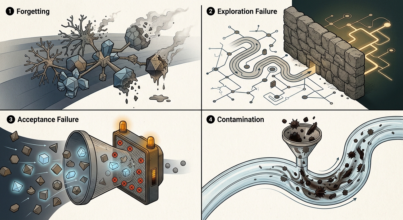
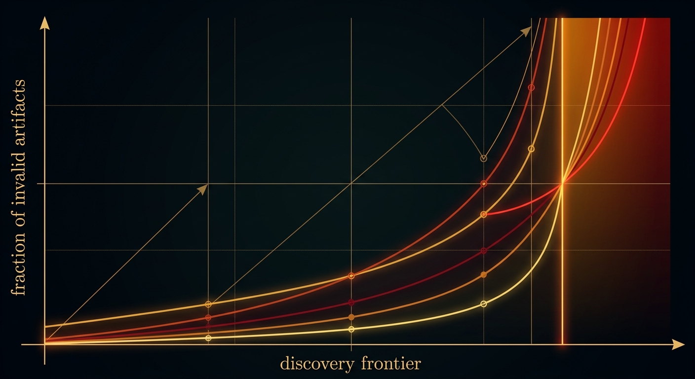
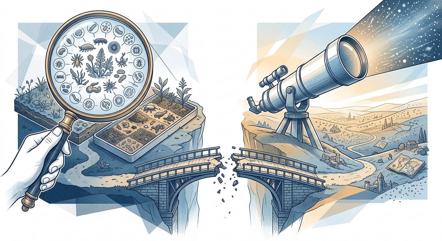
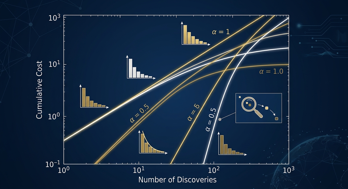
The preceding sections identify three barriers for autonomous NOVA: reachable support limits what can be discovered (Corollary 2), imperfect verification becomes more dangerous as new-valid mass shrinks (Corollary 4), and Zipf occupancy makes cumulative discovery costs grow superlinearly (Theorem 6). Human experts can intervene at each of these bottlenecks.

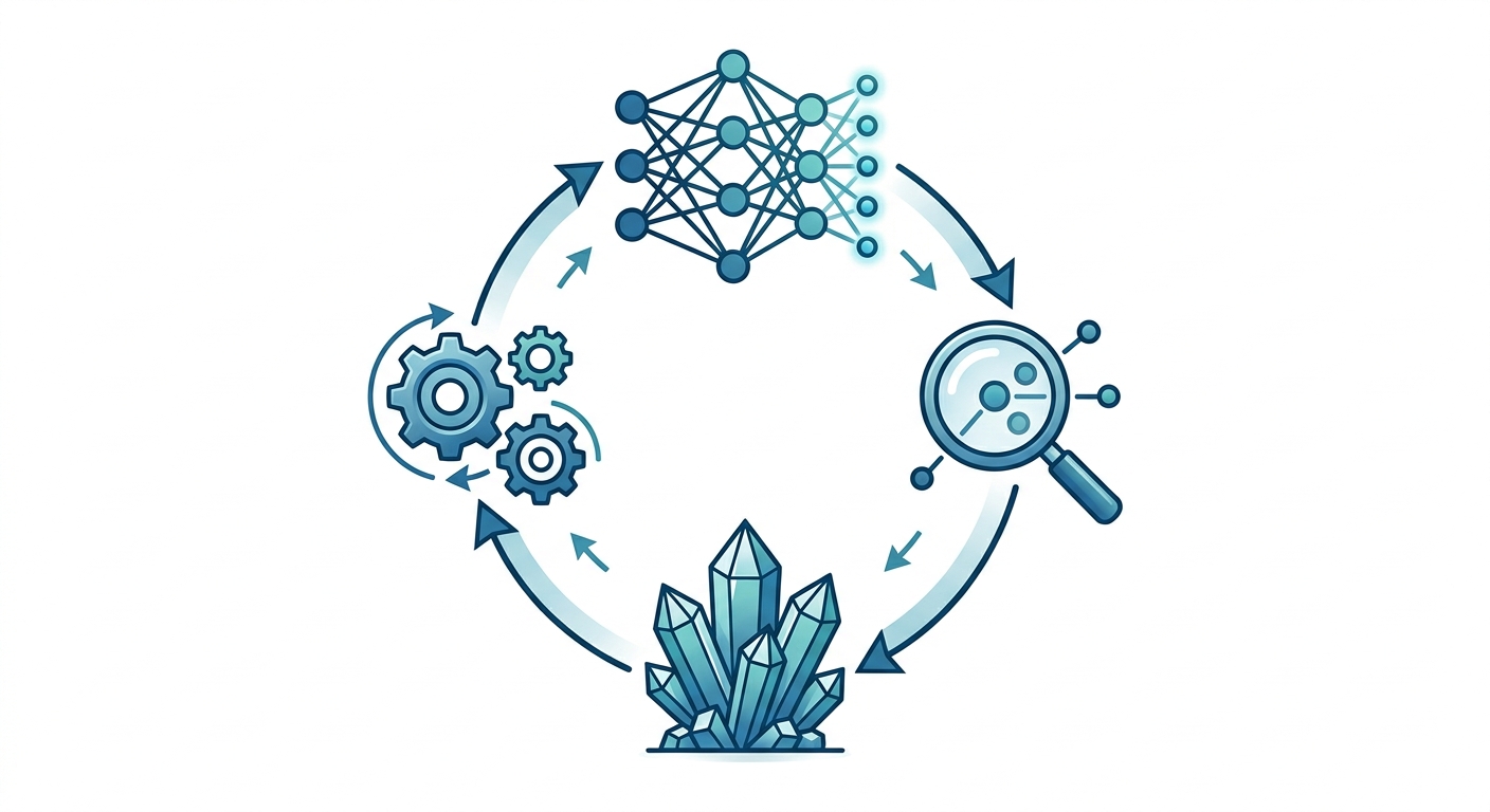
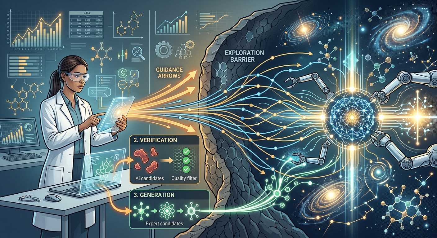
In the augmented NOVA loop, a human expert modifies $Q_t$ to a guided distribution $Q_t'$, the AI generates $N_{\text{AI}}$ candidates from $Q_t'$, the expert generates $N_H$ candidates from their own distribution $P_H$, and the combined candidates are verified.

Theorem 7

Sparse-Regime Human Amplification

In the sparse regime, the human amplification factor admits the first-order decomposition: $$\boxed{A_H = A_{\text{guide}} \cdot A_{\text{verify}} \cdot A_{\text{gen}}}$$ where: $$A_{\text{guide}} = \frac{M_t^{\text{new,guided}}}{M_t^{\text{new}}}, \qquad A_{\text{verify}} = \frac{r_{\text{eff},t}}{r_t}, \qquad A_{\text{gen}} = 1 + \frac{N_H\, \rho_{H,t}\, M_t^{\text{new},H}}{N_{\text{AI}}\, r_{\text{eff},t}\, M_t^{\text{new,guided}}}$$

Interpretive Remark

Theorem 7 separates three distinct human contributions:

$A_{\text{guide}}$ (Guidance): Raises the new-valid mass reached by AI generation. The expert redirects the model's sampling distribution toward unexplored regions of the knowledge space.

$A_{\text{verify}}$ (Verification): Improves acceptance of valid AI artifacts. Human review catches false negatives and provides higher-precision filtering.

$A_{\text{gen}}$ (Generation): Adds human-proposed candidates. The expert contributes novel artifacts from their own knowledge distribution, which may cover regions outside the AI's effective support.

Together, these factors suggest a copilot regime in which AI performs high-volume search within guided regions while the human provides frontier guidance, hypotheses, and difficult verification.

Theorem 8

Human-Guided Support Expansion

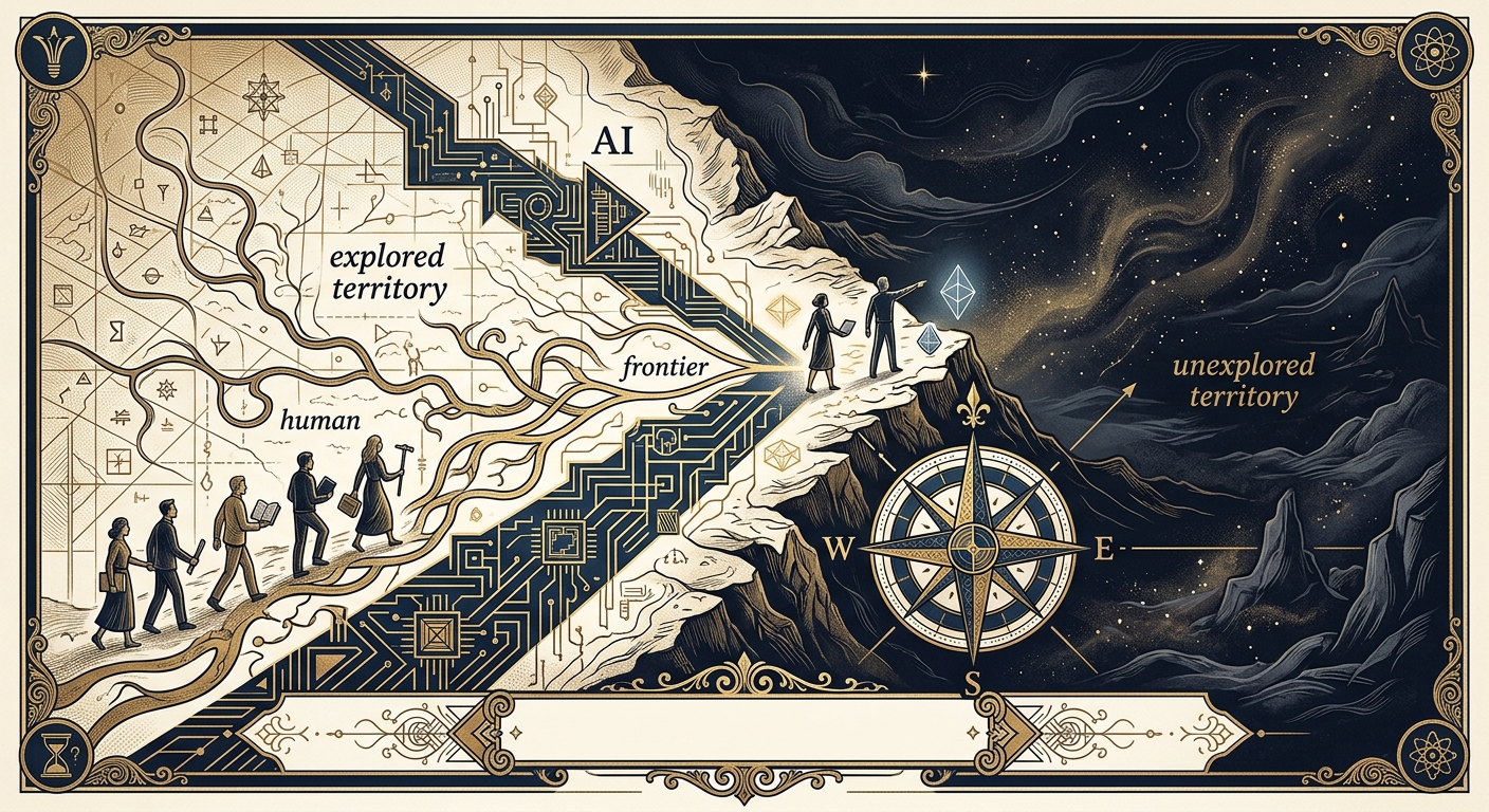
If human guidance changes $Q_t$ to $Q_t'$ such that $\mathcal{K} \cap \text{supp}(Q_t) \subsetneq \mathcal{K} \cap \text{supp}(Q_t')$, then the reachable valid set strictly expands. Hence guidance can break the autonomous exploration barrier.

Interpretive Remark

Theorem 8 is the formal counterpart to the qualitative observation emphasized by Klowden and Tao (2026): in frontier mathematical practice, AI systems are most effective when embedded in expert-guided workflows rather than treated as fully autonomous discovery engines. Guidance is especially central because it can change not only discovery probability within the current support, but also the support itself. This is the mechanism by which human expertise breaks through the exploration barrier that Corollary 2 establishes as a hard ceiling for autonomous systems.

Chapter Eight

Conclusions, Limitations, and Open Problems

Corresponds to Section 6 of the paper

NOVA shows that AI-driven discovery is a systems-level phenomenon, not merely generating more candidates. Discovery succeeds only when exploration, verification, accumulation, and retraining remain aligned. Otherwise, the loop can stall, forget, or contaminate itself.

Summary of Main Results

Theorem 1: Four sufficient conditions (C1-C4) for almost-sure coverage of a finite knowledge domain, with four named failure modes when violated.

Corollary 2: Autonomous discovery cannot exceed the initial generator's effective support without external intervention.

Corollary 4: The contamination trap: safe false-positive threshold $\delta_t^* = O(M_t^{\text{new}}/U_t)$ shrinks as the frontier advances.

Theorem 6: Cumulative cost scaling $R_{\text{cum}}(D) = \Theta(c_{\text{gen}} D^\alpha)$ under Zipf tail equivalence, proving diminishing returns.

Theorem 7: Human amplification decomposes as $A_H = A_{\text{guide}} \cdot A_{\text{verify}} \cdot A_{\text{gen}}$, with guidance most valuable near exploration barriers.

Theorem 8: Human guidance can strictly expand the reachable valid set, breaking the autonomous exploration barrier.

The paper identifies three open problems for future research:

Collaborative Discovery: How does effective missing mass scale with $m$ models with diverse supports, and can composition yield superlinear gains?
Verification Difficulty: Can we formalize how the difficulty of checking candidates (from mechanical proof checking to noisy experiments and subjective evaluation) limits the knowledge level achievable by autonomous NOVA?
Information Limits: For the subset $\mathcal{K}^* \subseteq \mathcal{K}$ discoverable from the initial data, model, and allowed NOVA operations, can $|\mathcal{K}^*|$ be bounded by the information that $D_0$ contains about $\mathcal{K}$, e.g., $|\mathcal{K}^*| \lesssim 2^{I(D_0;\mathcal{K})}$?

The strongest discovery systems are likely to be human-guided, verification-aware, and designed around the geometry of the unknown.

READ THE FULL PAPER →

Symbol	Meaning
\(M_t^{\text{new}}\)	Model mass on historically undiscovered valid artifacts
\(A_t\)	Mass on already-discovered genuine artifacts
\(U_t\)	Mass on invalid candidates
\(r_t\)	True-positive rate of the verifier
\(\delta_t\)	False-positive rate of the verifier
\(G_t, B_t\)	Counts of genuine and invalid retained artifacts